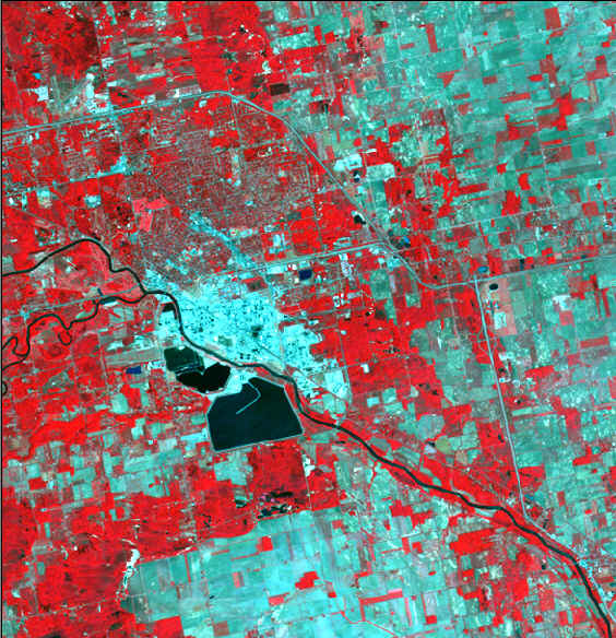
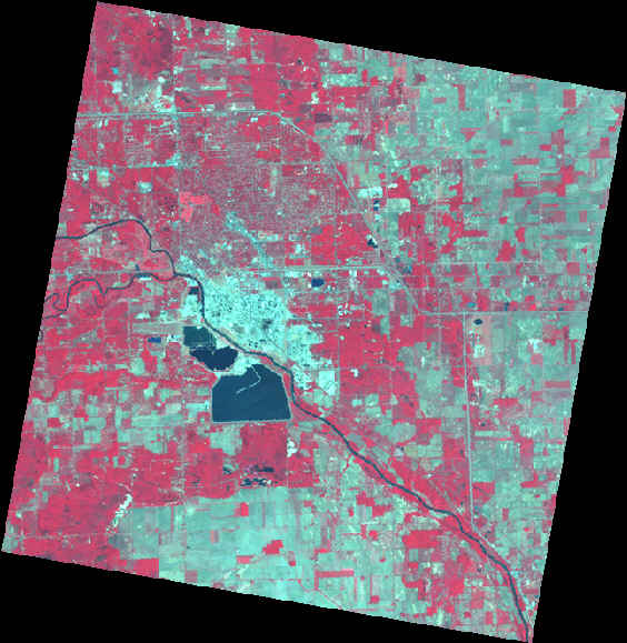
Image 1.  This is the original subset image before rectification, showing TM bands 4,3,2 (RGB).  Vegetation appears red because of its high response in the reflected infrared region of the spectrum (Band 4).  Ground control points were selected at various road intersections spread relatively evenly around the entire image area.

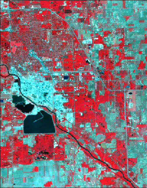
Image 2.  This is the original subset image after rectification, again with bands 4,3,2 (RGB).  As you can see, the orientation of the image has changed since it is now projected into UTM coordinates.  The contrast is different in this image because the black areas around the perimeter affect the contrast stretch applied in ERDAS.

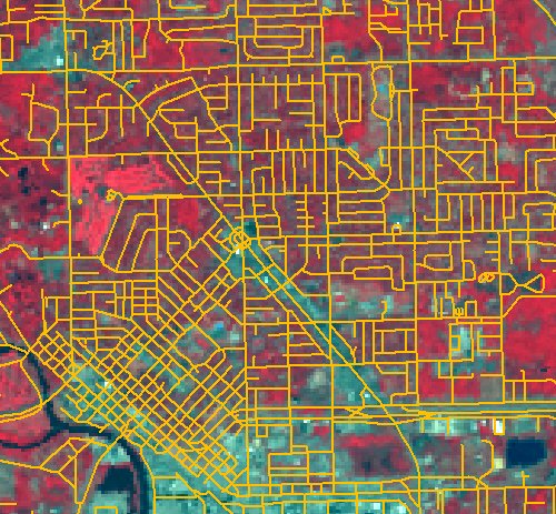
Image 3.  This is a subset of the rectified subset, which was done to eliminate the black areas around the perimeter.  This is the image that was spectrally enhanced and later classified.  The contrast has returned to normal with the removal of the black areas.

Image 4.  This image was created in ArcView GIS.  It shows a magnified portion of the rectified image with an overlaid GIS layer of the Midland street network.  The street information is part of a TIGER file that was downloaded from http://www.esri.com/.  Remember that the RMSE of 0.4640 was an indicator that this was a successful rectification.  An even better one is that the street network layer matches perfectly with the image underneath.  Notice how the streets outline features such as the Country Club, patches of forest, urban areas, etc.  The success of this rectification means that the image will now match up correctly with any GIS layer in the UTM projection.