|
Digital Image Processing Research Paper GEO 508 Digital Remote Sensing Dr. John Althausen Unsupervised
Classification of Spectrally Note: The images listed on
the right can also be viewed via links within the
|
Step One: Image Rectification Image rectification is an important procedure for many image processing applications. Simply put, it is the process of converting a raw image into a specified map projection (Sabins 266). The procedure involves the selection of distinguishable ground control points (GCP's) in the image, such as road intersections. These points are then assigned the appropriate reference information, such as latitude/longitude or UTM coordinates. This reference data can be obtained from existing map sheets or from fieldwork utilizing global positioning systems (GPS) (Sabins 266). After a certain number of GCP's have been entered and referenced, the computer program resamples the original pixels into the desired projection. The importance of rectification is that the image can now be used in conjunction with other data sets. For example, the rectified image could be opened in a Geographic Information Systems (GIS) program such as ArcView. Since the image is now in a certain map projection, it should line up perfectly with other projected layers of data, such as political boundaries, land use, soil types, road networks, drainage systems, etc. If the image was collected recently, the information could be used to update outdated GIS layers. The rectified image could also be used as the reference source for image-to-image registration. For this project, I used a Landsat-5 Thematic Mapper (TM) image of Michigan. Click here for more information about Landsat TM imagery. The characteristics of the TM image I used are summarized at the end of this section. After acquiring the image from Dr. John Althausen, I selected a subset image that included only the area (Midland) and the spectral bands I desired. Thematic Mapper images have seven bands of data, but I chose not to keep the thermal band (Band 6) because it is not particularly useful for classification. The next step was to find approximately 20 point locations such that I was able to 1) determine the Universal Transverse Mercator (UTM) coordinates of each point using a USGS topographic quad sheet, and 2) clearly see the point (such as a road intersection) on the image itself. I used the Midland North and Midland South quad sheets and a transparent UTM grid to determine the UTM coordinates (accurate to tens of meters) of each of the twenty points. Then I was ready to begin the rectification in ERDAS. After specifying the desired map projection information, I used the appropriate tools to:
Original Image Characteristics View Images of the Rectification Process |
Step Two: Spectral Enhancements The next step of this project
was to perform various spectral enhancements on the rectified image.
Spectral enhancements are modifications of the pixel values of an
image. They can be used to improve interpretability, reduce
information redundancy, and extract information from the data which is not
readily visible in its raw form. The two enhancements I utilized for
this project were principal components analysis and the tasseled cap
transformation. I made use of spectrally enhanced images because I
was interested in finding out if they could be used to generate a good
land cover classification map (typically the original multispectral bands
are used). Principal Components Analysis (PCA) Principal Components Analysis (PCA) is a spectral enhancement which can be used to compress the information content of a multispectral data set (Sabins 280). PCA uses mathematical algorithms to transform n bands of correlated data into n principal components which are uncorrelated, such that the coordinate axes of the components are mutually orthogonal (Corner). The first principal component (PC-1) describes most of the variation of the brightness values for the pixels of the original bands (Jensen 177). Subsequent components explain less and less of the data, with the final PC usually corresponding to atmospheric noise in the data rather than any ground features (Sabins 281). The main benefit of principal components analysis is that it can reduce the amount of data (bands) without losing much of the information and typically reducing redundancy (Jensen 172). For example, the three visible bands (1, 2, and 3) of TM images are usually highly correlated, meaning they look roughly the same and thus provide redundant information for classification purposes (Jensen 172). After running a principal components analysis on these three bands, we would find that the majority of the information contained within the three bands would be explained by PC-1. Thus, this one layer of data could replace the three original bands without much loss of information. In my project, I utilized two separate principal component enhancements. First, I ran a PCA on bands 1, 2, and 3 (the visible bands) of the image. Then I ran another PCA on bands 5 and 7 (the middle-infrared bands) because they too are typically highly correlated (Jensen 172). Later, when I was ready to classify the image, I used PC-1 from each of these two PCA's instead of having to use the 5 original bands. Since band 4 (near infrared) is less correlated to any of the others, I left it alone. Thus, I reduced the number of layers from six to three, with minimal loss of information. View PC-1 from the PCA of the three visible bands (1,2,3)
The Tasseled Cap Transformation is similar to PCA in that it attempts to reduce the amount of data layers (dimensionality) needed for interpretation or analysis. This enhancement uses mathematical equations to transform the original n multispectral bands into a new n-dimensional space. Thus, when a tasseled cap transformation is performed on six TM bands, six new layers are produced. It is the first two of these which contain the most information (95 to 98%) (Jensen 182). The other layers, while useful for some applications such as moisture study, explain much less of the data. One of the two more important layers is known as the soil brightness index (SBI). This index shows bare areas such as agricultural fields, beaches, and parking lots as the lightest features. The other is the green vegetation index (GVI), which is an indicator of vegetation status since it displays areas with healthy, green vegetation as the lightest feature. The name "tasseled cap" comes from the fact that when the greenness and brightness of a typical scene are plotted perpendicular to one another on a graph, the resulting plot usually looks like a cap (Jensen 183). I ran a tasseled cap transformation on the six TM bands of my image and then utilized the SBI and GVI for my classification. The use of these two layers along with the near-IR layer (band 4), should help to separate vegetation from bare features during the classification process (Center for Advanced Spatial Technologies). I decided not to use any further spectral enhancements because the addition of the SBI and GVI brought my total number of layers to five. I wanted to be sure to use fewer than six layers so that the dimensionality and processing time of the classification would be lower compared to a procedure that simply used the original six TM bands. View the Soil Brightness Index (SBI)
The final step of this portion of the project was to merge the five layers into one image which would then be classified. This was done in ERDAS using the "Layer Stack" algorithm. The following is a summary of the layers of data in the final enhanced image. Layer 1: PC-1 from TM bands 1, 2, and 3 |
Step Three: Unsupervised Classification In a multispectral image, each pixel has a spectral signature determined by the reflectance of that pixel in each of the spectral bands. Multispectral classification is an information extraction process that analyzes the spectral signatures and then assigns pixels to classes based on similar signatures (Sabins 283). For example, all of the pixels which represent an area of forested land on a TM image should have roughly the same spectral signature, with minor differences due to shadows, tree species, and health status. Classification procedures attempt to group together such similar pixels so that a GIS layer can be generated with each land cover type represented by a different class. The detail of the classes depends on the spectral and spatial resolution characteristics of the imaging system. Landsat TM imagery is usually good for creating a general land cover classification map. As explained earlier, my goal is to learn whether or not my combination of spectrally enhanced layers will also yield an accurate classification. Unsupervised classification is a method in which the computer searches for natural groupings of similar pixels called clusters (Jensen 231). The fewer clusters there are, the more the pixels within each cluster will vary in terms of spectral signature, and vice versa. In ERDAS, unsupervised classification is performed using an algorithm called the Iterative Self-Organizing Data Analysis Technique (ISODATA). For this algorithm, the analyst input the number of clusters desired and a confidence threshold. The computer will then build clusters iteratively, meaning that with each new iteration, the clusters become more and more refined. The iterations stop when the confidence level (or a maximum number of iterations specified by the user) is reached (Jensen 238). For example, if the user wants 30 clusters at 95% confidence, the computer will iteratively build the clusters until it is 95% confident that is has attained the best distribution of pixels into 30 clusters. After the clusters are built, the analyst must select the land cover classes (water, forest, etc.) and then assign each cluster to the appropriate class. For this step, it is important that the user have a good knowledge of the region being mapped, since he or she must decide what land cover the pixels of each cluster represent. Once all the clusters have been assigned to a class, the image of clusters can be recoded into a GIS layer which displays each land cover class with a different color. Once the spectral enhancements
were completed on my image of Midland, I performed an unsupervised
classification (using ISODATA) with 60 clusters and a 95% confidence
threshold. I set the maximum number of iterations at 15, but the
algorithm reached 95.2% confidence after only 13 iterations. The
result was an image with 60 groups of pixels each represented by a
different color. I was able to highlight each cluster one at a time
and then determine which of the classes it belonged to by interpreting the
original multispectral image. Then I changed the cluster color to an
appropriate one, for example, I made the water clusters blue.
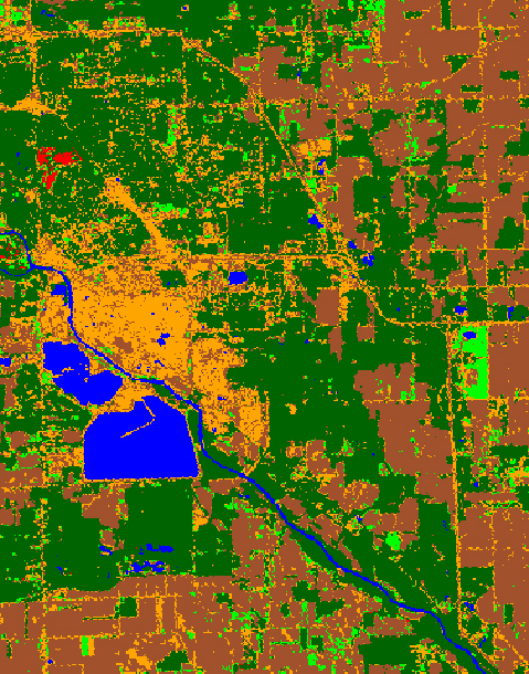
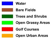
Finally, the image was recoded into the map shown below. The
following table lists the land cover classes I was able to
distinguish.
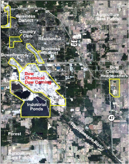
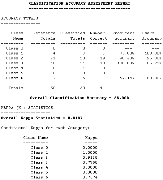
Overall, I think that the classification was very successful. The two classes that were easiest to separate from the others were the golf courses and water features. The manicured greens and fairways are what make the golf courses so distinguishable from other grassy areas, such as the grounds at Dow Corning Headquarters and various parks. As I expected, the residential areas of Midland were classified mostly as trees, with some patches of urban due to features such as church and school parking lots. The business and industrial districts are nicely shown as open urban areas, although they are speckled with pixels classified as bare fields, which are obviously misclassified. This occurred because some urban features have similar spectral signatures as bare fields and vice versa. However, I think that the spectrally enhanced layers did a pretty good job of separating these two classes, especially apparent in the fact that you can see the main roads (linear orange features) in the agricultural areas. The biggest problem with the classification was the issue of crops. As mentioned earlier, this image had almost exclusively bare fields because it was collected in June. Since there were so few areas with crops, it was too difficult to create a separate class called "crops" without creating a lot of misclassified pixels in other areas. The few crops in the image were grouped with either the trees/shrubs class or the grassy areas class. It is understandable, though, that some crops would appear similar to grass, especially if they were still very low to the ground, as would be expected in June. Other than this problem, the classification turned out very well, which will be confirmed in the next section regarding accuracy assessment. View a comparison of the classification map and the original image |
Conclusions This project has helped me learn a lot about several aspects of digital image processing. The results met my objective of finding out whether or not spectrally enhanced layers of data could be used to generate a good land cover classification map of the Midland area. As explained above, I feel that the unsupervised classification using the enhanced data was a success. I also think that with more than 50 random points selected, I could have achieved an even higher accuracy percentage. And although this project may not make any significant contributions to digital remote sensing research or a specific real world problem, the experience will definitely be valuable to me for the future GIS and remote sensing projects I may be involved with. References Center for Advanced Spatial
Technologies, University of Arkansas. Arkansas Gap
Analysis: Corner, Brian.
Principal Components Analysis. http://doppler.unl.edu/~bcorner/pca.html
Jensen, John R.
Introductory Digital Image Processing: A Remote Sensing
Perspective. 2nd Sabins, Floyd F.
Remote Sensing: Principles and Interpretation. 3rd
edition. New York: |